Excel tutorial: How to import and parse complicated data

 Image: Rob Schultz
Importing data into Excel from other sources can a real headache, especially if you’re copying and pasting from an Internet source. Data that’s exported from a mainframe; from another program such as Microsoft Access, Lotus, Word or Word Perfect, Adobe Acrobat; or from any other text-based source is, generally, an effortless process, because everything can be reduced to a simple ASCII text file.
Excel’s Import and Parsing options use a Wizard to guide you through these processes. Just follow the directions on the screens. Once the data is imported, the challenge is how to properly parse the data, especially if the information in each parsed field has multiple words, lots of punctuation, special characters, or other complications.
Import data
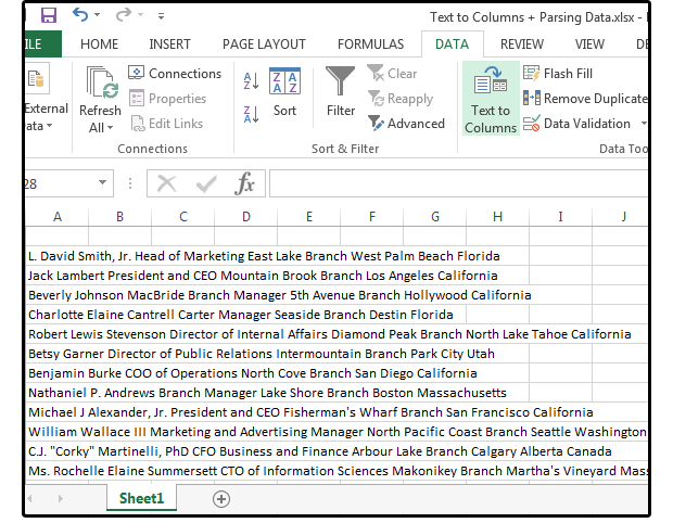
1. Open a blank Excel spreadsheet and use the instructions from “Excel pro tips: Importing and parsing data.” Note that all the information imports into one field, so you must parse the data to break up this string of text into separate fields. Note that parsing the data used in the reference article was a breeze because each field contained similar records.
2. For our example, we’ll just enter a dozen records, which you could edit manually in a few minutes. But the technique I’ll show you will work for editing thousands of records. Note: For the remainder of this article, let’s assume your spreadsheet has 1,000 records. The fields for this database are Name, Title, Branch Location, City, and State; that’s five columns (or fields).
 PC World / JD Sartain
All six fields imported into one column
Before you parse the database
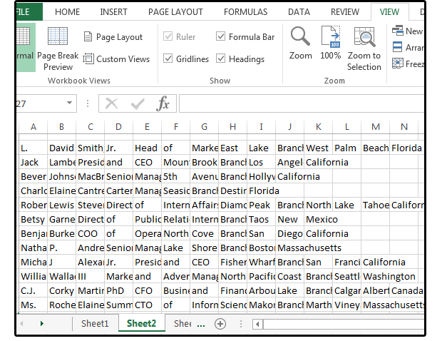
If you parse the database now, the results will be a mess, because some names have salutations or titles. Some have middle names or initials, some have suffixes and/or accreditations. In addition, the other fields contain between one and five words per record. And, because the only delimiter is the space, Excel creates a new field or column for each word. Cleaning up this mess involves several steps.
 PC World / JD Sartain
Parsed database before reorganization.
A. First, extract the last word
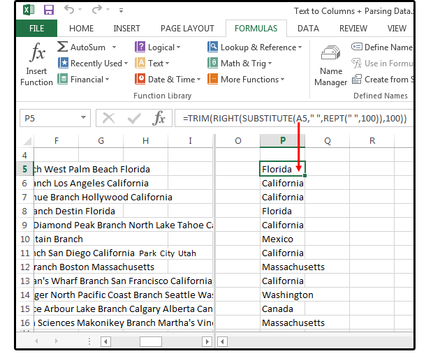
1. Let’s extract the last word in each string of text, then delete that word from the original database. In this case, it’s the state.
2. Move your cursor to cell P5 and enter this formula:
=TRIM(RIGHT(SUBSTITUTE(A5,” “,REPT(“ “,100)),100))
3. Copy the formula from P5 to P6 through P1000.
4. Next, highlight the range, select Copy, move one column to the right, and select Paste Values. If you fail to do this, the “state” information you extracted will change based on the new, parsed information in A5.
5. Delete column P.
 PC World / JD Sartain
Extract the last word in each string of text.
B. Delete the last word in each record/string of text
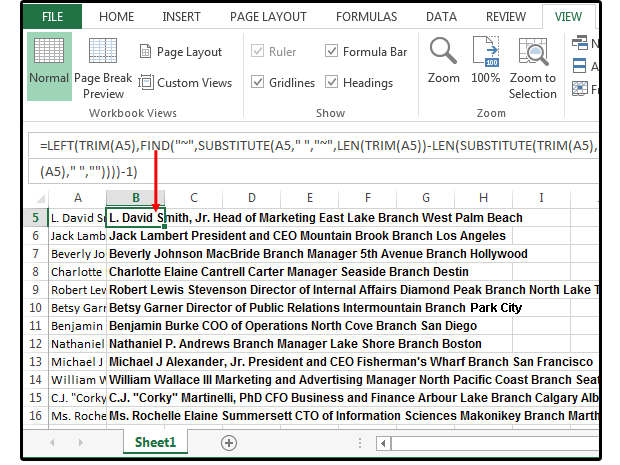
1. Move your cursor to column B and enter this formula:
=LEFT(TRIM(A5),FIND(“~”,SUBSTITUTE(A5,” “,”~”,LEN(TRIM(A5))-LEN(SUBSTITUTE(TRIM(A5),” “,””))))-1)
Note that all the data from A5 except the State is now in B5.
2. Copy this formula from B5 down to B6 through B1000.
3. Note that column B is now a formula, which must be converted to text.
4. Next, highlight the range (B5:B1000), select Copy, move one column to the right (column C), and select Paste Values.
5. Delete columns A and B. Everything moves to the left and the database is, once again, in column A.
 PC World – JD Sartain
Delete the last word in each string of text.
C. Use repetitive data to extract the city
The only consistent piece of information in this database is the word Branch. Let’s use that information to extract the city. There are several ways to perform this function. This is just one option.
1. First, let’s insert a character such as the plus (+) sign in our formula to simplify the Find & Replace procedure.
2. Move your cursor to the Home position.
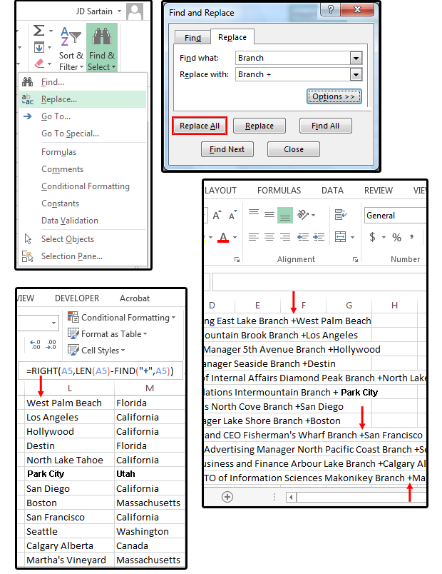
3. Under the Home tab, click the Find & Select button. Choose Replace from the list.
4. In the Find & Replace dialog enter the word Branch followed by a space in the Find What field box.
5. In the Replace With field box, enter the word Branch followed by a space and then a + sign.
6. To test your results, click the Find Next button, then click the Replace button. If you’re confident that your results will be accurate, just click the Replace All button.
7. Notice that Excel has placed a + sign between each city and the word Branch.
8. Next, enter this formula in cell M5: =RIGHT(A5,LEN(A5)-FIND(“+”,A5)).
9. Highlight the range and copy the formula in M5 down from M6 through M1000.
10. Note that column M is now a formula, which must be converted to text.
11. Next, highlight the range (M5:M1000), select Copy, move one column to the left (column L), and select Paste Values.
12. Delete column M (everything moves to the left), then expand column L to accommodate the longest city in the range.
 PC World / JD Sartain
Use repetitive data to extract the city.
D. Delete the city from the database string of text
1. Move your cursor to cell B5 and enter this formula:
=LEFT(A5, FIND(“+”, A5&”+”)-1)
Note that all the data from A5 except the City is now in B5
2. Copy this formula from B5 down to B6 through B1000.
3. Note that column B is now a formula, which must be converted to text.
4. Highlight the range (B5:B1000), select Copy, move one column to the right (column C), and select Paste Values.
5. Delete columns A and B. Everything moves to the left and the database is, once again, in column A.
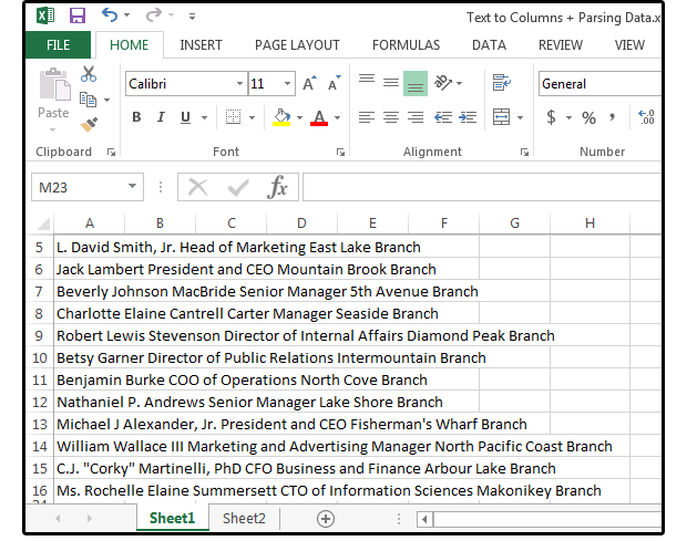
Note that the City has moved to column J and the State resides in column K.
 PC World / JD Sartain
Delete the city from the database string.
E. Before you parse, count the columns
Use this formula to count the number of columns/fields that Excel will need to parse your data.
Note: Just to be certain that you have enough working space on your spreadsheet to manipulate the data. You can always Insert or Delete columns and rows later.
1. Before you parse the data, move your cursor out to cell M5 and enter this formula:
=IF(LEN(TRIM(A5))=0,0,LEN(TRIM(A5))-LEN(SUBSTITUTE(A5,” “,””))+1).
2. Copy the formula from M5 (the first cell in your database) to M6 and down to the last cell in your database; e.g., M1000.
3. Highlight the range, select Copy, move one column to the right, and select Paste Values.
4. Next, delete column M (the formulas) and everything moves one column to the left.
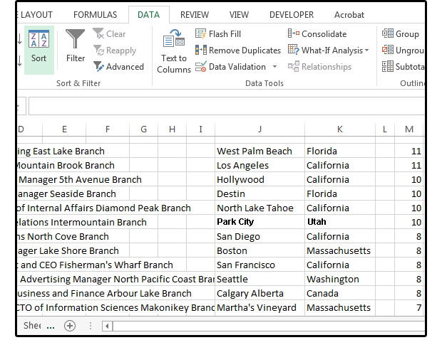
5. Sort the values in the new column M in Descending order (largest to smallest). The largest number in this range shows the number of columns you’ll need (to work with) when the data is parsed. In this case, it’s 11 columns: A through K, beginning on Row 5.
Note: Because columns J and K are already in use, and we need a few columns to work with, insert six new columns anywhere between B and K, pushing City and State out to columns P and Q.
 PC World / Jd Sartain
Use a formula to discover how many columns after parsing the data.
And now we parse the data
Next, parse the data using the Text to Columns Wizard.
1. Highlight the database (in this case, just column A).
2. Select Data > Text to Columns.
3. In the Text to Columns Wizard (Step 1), choose the Delimited button, then click Next.
 PC World / JD Sartain
Select Delimited from the Text to Columns Wizard Step 1
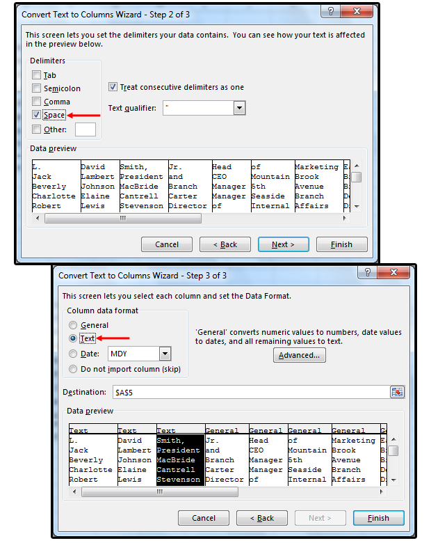
4. Check the Space box in the Wizard (Step 2), then click Next.
5. In Step 3, click the first column and, from the Column Data Format panel, click the Text button. Click the next column, and select the Text button again, and so forth to the end, then click Finish.
Note: If the column contains dates, click the Date button. For text, click the Text button; for numbers, click the General button. If you’re uncertain, use the General button for all the fields, because this button converts date fields to dates, numeric values to numbers, and everything else to text. Also note that you can select the Do Not Import Column (Skip) button to omit unnecessary fields.
Also note the cell address in the Destination field box. The default is the first cell in the first column of your highlighted range; e.g., $A$5. The default is normal. You can, however, select another cell address if, for example, you want the database located somewhere else on this sheet, another sheet, or in another workbook.
 PC World / JD Sartain
Choose the Space Delimiter and Text—or General—for your Column Data Format.
Next, organize the data
It’s still a mess, but it’s much better than it was! You now have six fields spread out across 11 columns. Why? Because the only logical delimiter was the space, so whenever Excel encountered a space, it created a new column. Now we have to put it all back together in a logical sequence.
A. Sort and CONCATENATE
1. Sort the database by column A. Note that the name field never exceeds four columns.
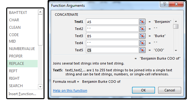
2. Move your cursor to L5. Select Formulas > Text > CONCATENATE. Under the Concatenate panel in the Function Arguments dialog window, there are multiple Text field boxes. Fill them out as follows:
Click A5 in Text1.Enter a space surrounded by quotation marks in Text2.Next, click B5 in Text3.Enter another space surrounded by quotation marks in Text4. Click C5 in Text5.Enter another space surrounded by quotation marks in Text6.Finally, click D5 in Text7, then click OK. Or, enter this formula in L5: =CONCATENATE(A5,” “,B5,” “,C5,” “,D5).
Some of the results will contain the entire name fields. Others will include the names plus part of the title.
4. Insert a new spreadsheet (New WS) and copy column L. Move to the new sheet and Paste Values into A5.
5. Also copy columns P (City) and Q (State) to columns D and E in the New WS.
 PC World / JD Sartain
Use the Concatenate function to join parsed fields
Note that there are only nine titles: CEO, CTO, CFO, COO, President, Senior Manager, Manager, Director, and Head. Some of the titles are attached to departments, such as Head of Marketing, Director of Public Relations, CTO of Information Sciences, etc. So, to be safe, we’ll add the applicable departments to our formulas as well.
Also Note: I don’t know the maximum number of Substitute functions allowed per formula. I do know that in 2003, it was limited to seven, but in Office versions 2007, 2010, and 2016 it’s more. For my purposes, I limit it to 10, because anything more than that gets too confusing to edit.
B. Use the SUBSTITUTE function to extract the titles and articles
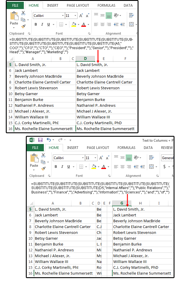
That said, enter the following formula in cell D5 of the New WS spreadsheet:
=SUBSTITUTE(SUBSTITUTE(SUBSTITUTE(SUBSTITUTE(SUBSTITUTE(SUBSTITUTE(SUBSTITUTE(SUBSTITUTE(SUBSTITUTE(SUBSTITUTE(A5,”COO”,””),”CFO”,””),”CTO”,””),”CEO”,””),”President”,””),”Senior”,””),”President”,””),”Head”,””),”Manager”,””),”Marketing”,””)
6. Enter this formula in cell G5:
=SUBSTITUTE(SUBSTITUTE(SUBSTITUTE(SUBSTITUTE(SUBSTITUTE(SUBSTITUTE(SUBSTITUTE(SUBSTITUTE(SUBSTITUTE(D5,”Internal Affairs”,””),”Public Relations”,””),”Business”,””),”Finance”,””),”Advertising”,””),”Information”,””),”Sciences”,””),”and”,””),”of”,””)
7. The first formula (which refers to A5) is entered in D5 and removes the titles. The second formula (which refers to D5) is entered in G5 and removes the departments and articles (and, of, etc.)
8. Copy the formula from G5 to G6 through G1000.
9. Highlight the range, select Copy, go to cell A5, and select Paste Values. Now you have the names separated from the titles.
10. Delete columns D and G.
 PC World / JD Sartain
Use the SUBSTITUTE function to remove titles and articles
C. CONCATENATE the remaining fields
1. Return to the original parsed database. The fields stretch out from A5 through K5.
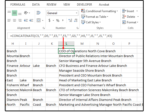
2. Move your cursor to L5 and enter this formula: =CONCATENATE(C5,” “,D5,” “,E5,” “,F5,” “,G5,” “,H5,” “,I5,” “,J5,” “,K5). This function reunites the titles and branches.
3. Copy the formula in L5 to L6 through L1000.
4. Next, move your cursor to cell R5 and enter this formula: =TRIM(RIGHT(SUBSTITUTE(TRIM(L5),” “,REPT(“ “,60)),180))
Important note: These two formulas also work for this step:
=MID(L5,(LEN(R5)+2),99)
=IF(ISERROR(SEARCH(R5,L5,1)),L5,RIGHT(L5,LEN(L5)-LEN(R5)))
5. Copy this formula in R5) to R6 through R1000. And now you have the branch information.
6. Highlight R5 through R1000 and select Copy. Move to the New WS spreadsheet and Paste Values into column C.
 PC World / JD Sartain
Extract the Branch information from the database
D. Extract title, and done
All that’s left to do now is to extract the titles and copy them to the New WS.
1. Move your cursor to cell T5. (Note that the cell locations are arbitrary).
2. Enter this formula: =SUBSTITUTE(L5,R5,””)
3. Copy the formula from T5 down to T6 through T1000.
4. Notice that the titles are extracted from the combined titles and branch names in column L.
 PC World / JD Sartain
Extract the titles from the combined fields in column L
5. Copy the titles from column T into column B of the New WS. Be sure to use Paste > Special > Values.
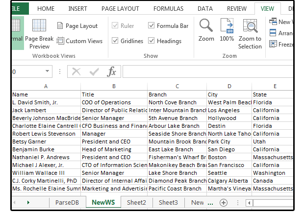
Now all the columns with multiple words are separated into the correct fields so you can work with the data by field—create a mailing list for Mail Merge, print envelopes or labels, merge to Outlook, or use the information in another database.
 PC World / JD Sartain
The completely parsed database


