Excel Date and Time functions: WEEKNUM, ISOWEEKNUM, WORKDAY, WORKDAY.INTL

Excel’s Date & Time functions ease the workload for bookkeepers, project planners, HR departments, and other jobs where time is money. The four functions covered here—ISOWEEKNUM, WEEKNUM, WORKDAY, WORKDAY.INTL—are complicated, so we’ll walk you through detailed instructions and examples.

Note: Each function is defined first, followed by the function’s arguments (the values that functions use to perform calculations), followed by the function’s syntax—how a formula is arranged, which includes the function’s name and its arguments.

Remember: Arguments are always surrounded by parentheses, and individual arguments are separated by commas.

Week-numbering functions

Currently, there are only three main week numbering systems in use worldwide, and each has its own unique qualities. Here are the systems and the Excel functions that work with them. 

WEEKNUM uses an optional second argument to define weeks beginning on specific days.ISOWEEKNUM() works with the ISO Week system, defined by ISO (International Organization for Standardization).In the Manual Method of week numbering, the first week begins on January 1st, the second week begins on January 8th, and so on, ending with a week 53 that has only one or two days for the leap years.

WEEKNUM()

The arguments for this function are:

Serial_number: any date within the week: For example, it can be a cell reference that contains a date, a date entered with the DATE function, or a date calculated from another formula.

Return_type (optional): a number that determines which day the week begins (the default is type 1, the week beginning on Sunday).

The syntax looks like this: WEEKNUM(serial_number,[return_type])

Result: The answer returns a week number value between 1 and 54

Return Types-Week begins on:

1 or 17 (or omitted): Sunday 

2 or 11: Monday 

12: Tuesday 

13: Wednesday 

14: Thursday 

15: Friday 

16: Saturday 

21: Monday (used in the ISO Week Number function)

Here’s how to set up a formula with WEEKNUM:

1. Enter 10 or 12 random dates in cells A4 to A15.

2. Move your cursor to B4. Go to Formulas > Date & Time and select WEEKNUM from the dropdown list.

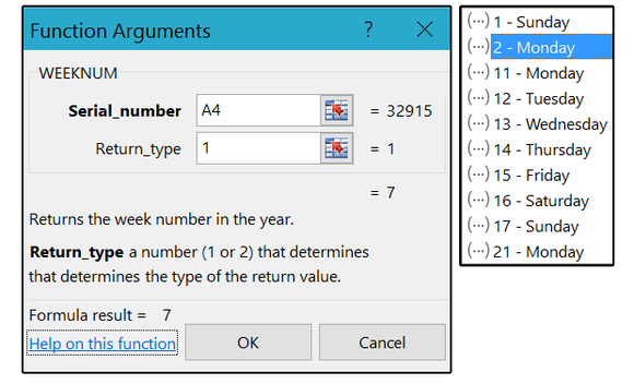
Note: When the function is entered, if you press any key (such as the space bar) after the last argument, Excel provides a popup menu that lists the 10 options above. Select the appropriate code from the list and press Enter.

JD Sartain

3. In the Function Arguments dialog window, click your cursor in the Serial Number field (it should already be positioned in this field box), then click cell A4 (the first date in your column of random dates).

4. The week number appears in cell B4. Notice the formula (syntax) appears in the Formula Bar above.

5. Copy the formula from cell B4 to B5 through B15.

JD Sartain

ISOWEEKNUM()

The ISO (International Organization for Standardization) week-numbering system is used primarily by bookkeepers, timekeepers, accountants, engineers, human resources, government, and information systems for calculating fiscal years. Basically, this system defines each year by the week instead of days or months. It works on the Gregorian calendar by defining a notation for the ordinal weeks of the year. In short, the ISO week numbering system has 52 or 53 full weeks, with 364 or 371 days, respectively. Weeks begin on Monday, and the week number 1 is assigned to the first week in each year that contains a Thursday.

Note: Microsoft introduced this function in Excel 2013. In earlier versions of Excel, the WEEKNUM function was the only way to get an Excel formula to return a week number.

The arguments for this function are:

Date: a valid date (as a date or an Excel serial number)The syntax looks like this: =ISOWEEKNUM(date)Result: The answer returns a value (or week number) between 1 and 53.

1. Enter 10 or 12 random dates in column A from A4 to A15.

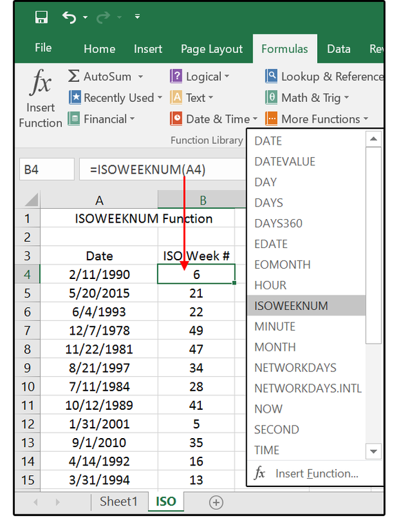
2. Move your cursor to B4. Go to Formulas > Date & Time and select ISOWEEKNUM from the dropdown list.

JD Sartain

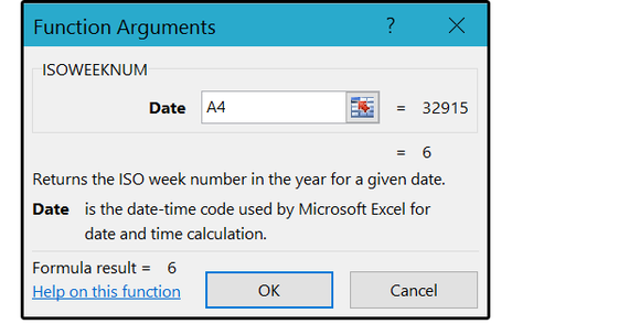
3. In the Function Arguments dialog window, click your cursor in the Date field (it should already be positioned in this field box), then click cell A4 (the first date in your column of random dates).

4. The ISO week number appears in cell B4. Notice the formula (syntax) appears in the Formula Bar (up top).

5. Copy the formula from cell B4 to B5 through B15.

JD Sartain

WORKDAY()

Use the WORKDAY function to calculate delivery dates, due dates, future dates, or random dates in a range. You can also calculate a series of dates by workdays, or get a starting date based on a target date, excluding certain days such as holidays, comp days, or non-working days.

Note that we use a positive number to calculate future dates and a negative number to calculate past dates.

The arguments for this function are:

start_date: the date from which to start.days: the working days before or after start_date.holidays: an optional list of dates defined as non-working days.

The syntax looks like this: =WORKDAY (start_date,days,[holidays])

The answer returns a serial number that represents a specific date. 

Notes: The WORKDAY function does not include the start_date “date” as a work day when it calculates the end_date. Also, the WORKDAY function does NOT include “normal” weekend days; that is, Saturdays and Sundays.

1. Enter the following field/column headers over columns A, B, C, D, and E, respectively: Start Date, Days, Results, and Holidays (centered and merged over D and E).

2. Enter some random dates in columns A and some random numbers (for number of days) in column B.

3. Enter your company’s holidays (names and dates) into columns D and E.

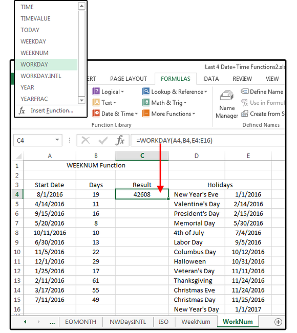
4. Position your cursor in cell C4 (Result column). Go to Formulas > Date & Time, then select the WORKDAY function from the dropdown list.

JD Sartain

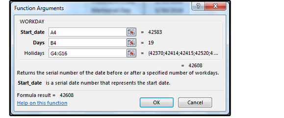
5. In the Function Arguments dialog box, click inside the Start_Date field box, then click your cursor in cell A4.

6. Press the Tab key down to the Days field box and click your cursor in cell B4.

7. Press the Tab key down to the field box Holidays, then select/highlight the cells that contain your company’s holiday dates: E4 through E16. Click OK.

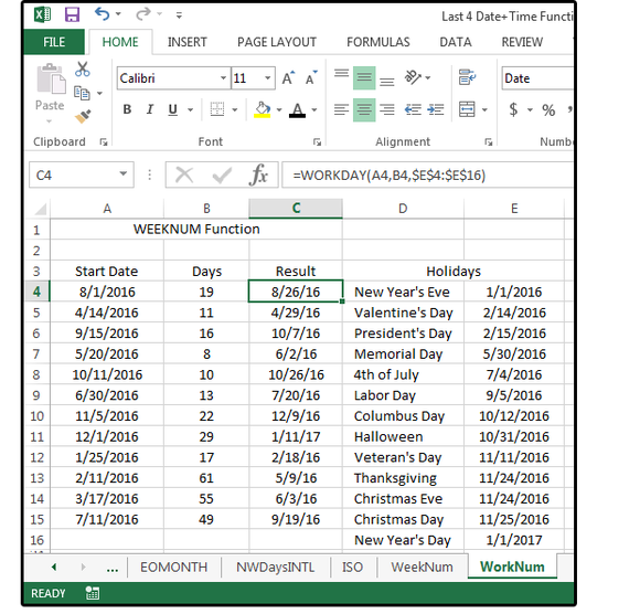
Notice the formula is listed in the Formula Bar: =WORKDAY(A4,B4,E4:E16). A4 is Start_Date, B4 is the number of Days, and E4 through E16 is the range of holidays.

Important: Before you copy this formula from cell C4 down to C5 through C15, be SURE to use the function key F4 to make the Holiday cells absolute: =WORKDAY(A4,B4,$E$4:$E$16) so the days in the Holidays range are always the same (E4 through E16).

JD Sartain

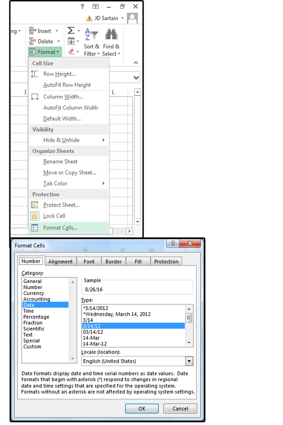
8. Next, from Home > Format, select Format cells from the dropdown menu. Choose a Date format from the Date category, then click OK.

9. Copy the formula/date in C4 to C5 through C15.

JD Sartain

10. Using this formula, you can see, for example, there are 19 “working” days between August 1 and August 26th (B4) and 11 “working” days between April 14th and April 29th (B5).

JD Sartain

WORKDAY.INTL()

The primary difference between WORKDAY.INTL and WORKDAY is that with the INTL function, you can customize which days of the week are weekends. This function was added to the formulas menu in Excel 2010; therefore, it is not available in previous versions.

The arguments for this function are:

start_date: the starting datedays: the ending dateweekend days [optional]: use this parameter to define weekend daysholidays [optional]: a defined list of holiday dates; i.e., non working days

The syntax looks like this: =WORKDAY.INTL (start_date,days,[weekend], [holidays])

Result: Returns the next or previous working date based on data entered.

Remember to use a positive number for future dates and a negative number for past dates. Also, enter the holidays as a range of cells where you’ve specified the actual holiday dates, or as a list of serial numbers that represent the actual dates of the holidays.

1. Use the same spreadsheet as above.

2. Delete the WORKDAY functions in column C.

3. Use the same holiday range as above; that is, E4 through E16.

4. Use the following Weekend Days code numbers below to define your weekend days. If you leave this parameter blank (or unidentified), it defaults to number 1.

Number Weekend days

1 Saturday, Sunday

2 Sunday, Monday

3 Monday, Tuesday

4 Tuesday, Wednesday

5 Wednesday, Thursday

6 Thursday, Friday

7 Friday, Saturday

11 Sunday only

12 Monday only

13 Tuesday only

14 Wednesday only

15 Thursday only

16 Friday only

17 Saturday only

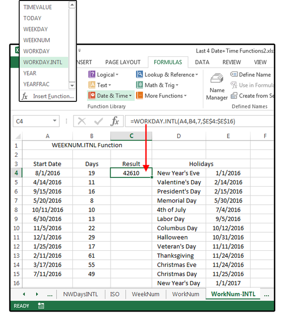
5. Position your cursor in cell C4 (Result column). From the Formulas tab> Date & Time button, select the WORKDAY.INTL function from the dropdown list.

JD Sartain

6. In the Function Arguments dialog box, click inside the Start_Date field box, then click your cursor in cell A4.

7. Press the Tab key down to the Days field box and click your cursor in cell B4.

8. Press the Tab key down to the Weekend field box and enter the number from the above list that corresponds with your weekend days. I selected number 7, for Fridays and Saturdays, so the result will differ from the prior example, where we used the default weekend days of Saturday and Sunday. 

9. Press the Tab key down to the field box Holidays, then select the cells that contain your company’s holiday dates: E4 through E16. Click OK.

Notice the formula in the Formula Bar: =WORKDAY.INTL(A4,B4,7,E4:E16). A4 is Start_Date, B4 is the number of Days, 7 is the code for the weekend days Friday and Saturday, and E4 through E16 is the range of holidays.

Don’t forget to use the function key F4 to make the Holiday cells absolute: =WORKDAY.INTL(A4,B4,7,$E$4:$E$16) so the days in the Holidays range are always the same (E4 through E16).

JD Sartain

8. Next, from Home > Format, select Format cells from the dropdown menu. Choose a Date format from the Date category, then click OK.

9. Copy the formula/date in C4 to C5 through C15. 

JD Sartain